Published On:Wednesday, 14 December 2011
Posted by Muhammad Atif Saeed
Sampling
Populations, Samples, Parameters, and Statistics
The field of inferential statistics enables you to make educated guesses about the numerical characteristics of large groups. The logic of sampling gives you a way to test conclusions about such groups using only a small portion of its members.A population is a group of phenomena that have something in common. The term often refers to a group of people, as in the following examples:
- All registered voters in Crawford County
- All members of the International Machinists Union
- All Americans who played golf at least once in the past year
- All widgets produced last Tuesday by the Acme Widget Company
- All daily maximum temperatures in July for major U.S. cities
- All basal ganglia cells from a particular rhesus monkey
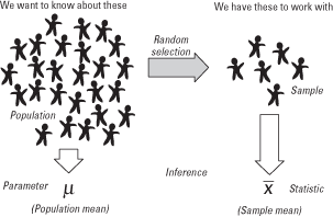
A parameter is a characteristic of a population. A statistic is a characteristic of a sample. Inferential statistics enables you to make an educated guess about a population parameter based on a statistic computed from a sample randomly drawn from that population (see Figure 1).
Figure 1. Illustration of the relationship between samples and populations.
Sampling Distributions
Continuing with the earlier example, suppose that ten different samples of 100 people were drawn from the population, instead of just one. You would not expect the income means of these ten samples to be exactly the same, because of sampling variability (the tendency of the same statistic computed from a number of random samples drawn from the same population to differ).Suppose that the first sample of 100 magazine subscribers was “returned” to the population (made available to be selected again), another sample of 100 subscribers was selected at random, and the mean income of the new sample was computed. If this process were repeated ten times, it might yield the following sample means:
| 27,500 | 27,192 | 28,736 | 26,454 | 28,527 |
| 28,407 | 27,592 | 27,684 | 28,827 | 27,809 |
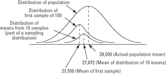
You can estimate the mean of this sampling distribution by summing the ten sample means and dividing by ten, which gives a distribution mean of 27,872.8. Suppose that the mean income of the entire population of subscribers to the magazine is $28,000. (You usually do not know what it is.) You can see in Figure 1 that the first sample mean ($27,500) was not a bad estimate of the population mean and that the mean of the distribution of ten sample means ($27,872) was even better.
Figure 1. Estimation of the population mean becomes progressively more accurate as more samples are taken.
Random and Systematic Error
Two potential sources of error occur in statistical estimation—two reasons a statistic might misrepresent a parameter. Random error occurs as a result of sampling variability. The ten sample means in the preceding section differed from the true population mean because of random error. Some were below the true value; some above it. Similarly, the mean of the distribution of ten sample means was slightly lower than the true population mean. If ten more samples of 100 subscribers were drawn, the mean of that distribution—that is, the mean of those means—might be higher than the population mean.Systematic error or bias refers to the tendency to consistently underestimate or overestimate a true value. Suppose that your list of magazine subscribers was obtained through a database of information about air travelers. The samples that you would draw from such a list would likely overestimate the population mean of all subscribers' income because lower-income subscribers are less likely to travel by air and many of them would be unavailable to be selected for the samples. This example would be one of bias.
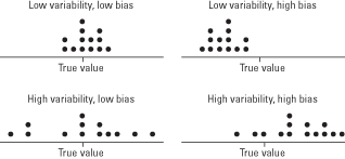
In Figure 1, both of the dot plots on the right illustrate systematic error (bias). The results from the samples for these two situations do not have a center close to the true population value. Both of the dot plots on the left have centers close to the true population value.
Figure 1. Random (sampling) error and systematic error (bias) distort the estimation of population parameters from sample statistics.
Central Limit Theorem
If the population of all subscribers to the magazine were normal, you would expect its sampling distribution of means to be normal as well. But what if the population were non-normal? The central limit theorem states that even if a population distribution is strongly non-normal, its sampling distribution of means will be approximately normal for large sample sizes (over 30). The central limit theorem makes it possible to use probabilities associated with the normal curve to answer questions about the means of sufficiently large samples.According to the central limit theorem, the mean of a sampling distribution of means is an unbiased estimator of the population mean.


Example 1
If the population mean of number of fish caught per trip to a particular fishing hole is 3.2 and the population standard deviation is 1.8, what are the mean and standard deviation of the sampling distribution for samples of size 40 trips?
Properties of the Normal Curve
Known characteristics of the normal curve make it possible to estimate the probability of occurrence of any value of a normally distributed variable. Suppose that the total area under the curve is defined to be 1. You can multiply that number by 100 and say there is a 100 percent chance that any value you can name will be somewhere in the distribution. ( Remember : The distribution extends to infinity in both directions.) Similarly, because half the area of the curve is below the mean and half is above it, you can say that there is a 50 percent chance that a randomly chosen value will be above the mean and the same chance that it will be below it.It makes sense that the area under the normal curve is equivalent to the probability of randomly drawing a value in that range. The area is greatest in the middle, where the “hump” is, and thins out toward the tails. That is consistent with the fact that there are more values close to the mean in a normal distribution than far from it.
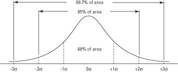
When the area of the standard normal curve is divided into sections by standard deviations above and below the mean, the area in each section is a known quantity (see Figure 1). As explained earlier, the area in each section is the same as the probability of randomly drawing a value in that range.
Figure 1. The normal curve and the area under the curve between σ units.

Sections of the curve above and below the mean may be added together to find the probability of obtaining a value within (plus or minus) a given number of standard deviations of the mean (see Figure 2). For example, the amount of curve area between one standard deviation above the mean and one standard deviation below is 0.3413 + 0.3413 = 0.6826, which means that approximately 68.26 percent of the values lie in that range. Similarly, about 95 percent of the values lie within two standard deviations of the mean, and 99.7 percent of the values lie within three standard deviations.
Figure 2. The normal curve and the area under the curve between σ units.

Example 1
A normal distribution of retail-store purchases has a mean of $14.31 and a standard deviation of 6.40. What percentage of purchases were under $10? First, compute the z-score:
Table 2 in "Statistics Tables" gives the area of the curve below z—in other words, the probability of obtaining a value of z or lower. Not all standard normal tables use the same format, however. Some list only positive z-scores and give the area of the curve between the mean and z. Such a table is slightly more difficult to use, but the fact that the normal curve is symmetric makes it possible to use it to determine the probability associated with any z-score, and vice versa.
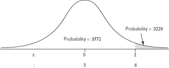
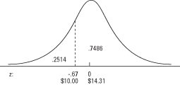
To use Table 2 (the table of standard normal probabilities) in "Statistics Tables," first look up the z-score in the left column, which lists z to the first decimal place. Then look along the top row for the second decimal place. The intersection of the row and column is the probability. In the example, you first find –0.6 in the left column and then 0.07 in the top row. Their intersection is 0.2514. The answer, then, is that about 25 percent of the purchases were under $10 (see Figure 3).
What if you had wanted to know the percentage of purchases above a certain amount? Because Table gives the area of the curve below a given z, to obtain the area of the curve above z, simply subtract the tabled probability from 1. The area of the curve above a z of –0.67 is 1 – 0.2514 = 0.7486. Approximately 75 percent of the purchases were above $10.
Just as Table can be used to obtain probabilities from z-scores, it can be used to do the reverse.
Figure 3. Finding a probability using a z-score on the normal curve.
Example 2
Using the previous example, what purchase amount marks the lower 10 percent of the distribution?Locate in Table the probability of 0.1000, or as close as you can find, and read off the corresponding z-score. The figure that you seek lies between the tabled probabilities of 0.0985 and 0.1003, but closer to 0.1003, which corresponds to a z-score of –1.28. Now, use the z formula, this time solving for x:

Normal Approximation to the Binomial
Some variables are continuous—there is no limit to the number of times you could divide their intervals into still smaller ones, although you may round them off for convenience. Examples include age, height, and cholesterol level. Other variables are discrete, or made of whole units with no values between them. Some discrete variables are the number of children in a family, the sizes of televisions available for purchase, or the number of medals awarded at the Olympic Games.A binomial variable can take only two values, often termed successes and failures. Examples include coin tosses that come up either heads or tails, manufactured parts that either continue working past a certain point or do not, and basketball tosses that either fall through the hoop or do not.
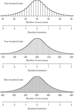
You discovered that the outcomes of binomial trials have a frequency distribution, just as continuous variables do. The more binomial trials there are (for example, the more coins you toss simultaneously), the more closely the sampling distribution resembles a normal curve (see Figure 1). You can take advantage of this fact and use the table of standard normal probabilities (Table 2 in "Statistics Tables") to estimate the likelihood of obtaining a given proportion of successes. You can do this by converting the test proportion to a z-score and looking up its probability in the standard normal table.
Figure 1. As the number of trials increases, the binomial distribution approaches the normal distribution.
μ = nπ
and the standard deviation is 
Example 1
Assuming an equal chance of a new baby being a boy or a girl (that is, π = 0.5), what is the likelihood that more than 60 out of the next 100 births at a local hospital will be boys?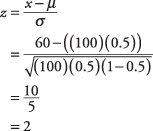
Figure 2. Finding a probability using a z-score on the normal curve.
