Published On:Wednesday, 14 December 2011
Posted by Muhammad Atif Saeed
Principles of Testing
Stating Hypotheses
One common use of statistics is the testing of scientific hypotheses. First, the investigator forms a research hypothesis that states an expectation to be tested. Then the investigator derives a statement that is the opposite of the research hypothesis. This statement is called the null hypothesis (in notation: H0). It is the null hypothesis that is actually tested, not the research hypothesis. If the null hypothesis can be rejected, that is taken as evidence in favor of the research hypothesis (also called the alternative hypothesis, Ha in notation). Because individual tests are rarely conclusive, it is usually not said that the research hypothesis has been “proved,” only that it has been supported.An example of a research hypothesis comparing two groups might be the following:
Fourth-graders in Elmwood School perform differently in math than fourth-graders in Lancaster School. This could be measured by comparing the means of these groups.Or in notation: Ha : μ1 ≠ μ2 or sometimes: Ha : μ1 – μ2 ≠ 0
The null hypothesis would be: Fourth-graders in Elmwood School perform the same in math as fourth-graders in Lancaster School.In notation: H0: μ1 = μ2 or: H0: μ1 – μ2 = 0
Some research hypotheses are more specific than that, predicting not only a difference but a difference in a particular direction. These are often described as one-sided tests: Fourth-graders in Elmwood School are better in math than fourth-graders in Lancaster School. In notation: Ha : μ1 > μ2 or: Ha : μ1 – μ2 > 0
The Test Statistic
Hypothesis testing involves the use of distributions of known area, like the normal distribution, to estimate the probability of obtaining a certain value as a result of chance. The researcher is usually testing to see if the probability will be low because that means it is likely that the test result was not a mere coincidence but occurred because the researcher's theory is correct. It could mean, for example, that it is probably not just bad luck but faulty packaging equipment that caused you to get a box of raisin cereal with only five raisins in it.Only two outcomes of a hypothesis test are possible: Either the null hypothesis is rejected, or it is not. You have seen that values from normally distributed populations can be converted to z-scores and their probabilities looked up in Table 2 in "Statistics Tables." The z-score is one kind of test statistic that is used to determine the probability of obtaining a given value. In order to test hypotheses, you must decide in advance what number to use as a cutoff for whether the null hypothesis will be rejected. This number is sometimes called the critical or tabled value because it is looked up in a table. It represents the level of probability that you will use to test the hypothesis. If the computed test statistic has a smaller probability than that of the critical value, the null hypothesis will be rejected.
For example, suppose you want to test the theory that sunlight helps prevent depression. One hypothesis derived from this theory might be that hospital admission rates for depression in sunny regions of the country are lower than the national average. Suppose that you know the national annual admission rate for depression to be 17 per 10,000. You intend to take the mean of a sample of admission rates from hospitals in sunny parts of the country and compare it to the national average.
Your research hypothesis is:
The mean annual admission rate for depression from the hospitals in sunny areas is less than 17 per 10,000.In notation: Ha : μ1 < 17 per 10,000
The null hypothesis is: The mean annual admission rate for depression from the hospitals in sunny areas is equal to 17 per 10,000.In notation: H0: μ1 = 17 per 10,000
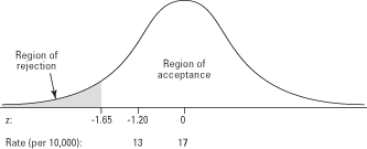
Your next step is to choose a probability level for the test. You know that the sample mean must be lower than 17 per 10,000 in order to reject the null hypothesis, but how much lower? You settle on a probability level of 5 percent. That is, if the mean admission rate for the sample of sunny hospitals is so low that the chance of obtaining that rate from a sample selected at random from the national population is less than 5 percent, you will reject the null hypothesis and conclude that there is evidence to support the hypothesis that exposure to the sun reduces the incidence of depression.Next, you look up the critical z-score—the z-score that corresponds to your chosen level of probability—in the standard normal table. It is important to remember which end of the distribution you are concerned with. Table 2 in "Statistics Tables" lists the probability of obtaining a given z-score or lower. That is, it gives the area of the curve below the z-score. Because a computed test statistic in the lower end of the distribution will allow you to reject your null hypothesis, you look up the z-score for the probability (or area) of 0.05 and find that it is –1.65. If you were hypothesizing that the mean in sunny parts of the country is greater than the national average, you would have been concerned with the upper end of the distribution instead and would have looked up the z-score associated with the probability (area) of 0.95, which is z = 1.65.
The critical z-score allows you to define the region of acceptance and the region of rejection of the curve (see Figure 1). If the computed test statistic is below the critical z-score, you can reject the null hypothesis and say that you have provided evidence in support of the alternative hypothesis. If it is above the critical value, you cannot reject the null hypothesis.
Figure 1. The z-score defines the boundary of the zones of rejection and acceptance.
 Suppose that the mean admission rate for the sample of hospitals in sunny regions is 13 per 10,000 and suppose also that the corresponding z-score for that mean is –1.20. The test statistic falls in the region of acceptance; so you cannot reject the null hypothesis that the mean in sunny parts of the country is significantly lower than the mean in the national average. There is a greater than 5 percent chance of obtaining a mean admission rate of 13 per 10,000 or lower from a sample of hospitals chosen at random from the national population, so you cannot conclude that your sample mean could not have come from that population.
One- and Two-Tailed Tests
In the previous example, you tested a research hypothesis that predicted not only that the sample mean would be different from the population mean but that it would be different in a specific direction—it would be lower. This test is called a directional or one-tailed test because the region of rejection is entirely within one tail of the distribution.Some hypotheses predict only that one value will be different from another, without additionally predicting which will be higher. The test of such a hypothesis is nondirectional or two-tailed because an extreme test statistic in either tail of the distribution (positive or negative) will lead to the rejection of the null hypothesis of no difference.
Suppose that you suspect that a particular class's performance on a proficiency test is not representative of those people who have taken the test. The national mean score on the test is 74.
The research hypothesis is:
The mean score of the class on the test is not 74.Or in notation: Ha : μ ≠ 74
The null hypothesis is: The mean score of the class on the test is 74.In notation: H0: μ = 74
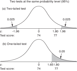
As in the last example, you decide to use a 5 percent probability level for the test. Both tests have a region of rejection, then, of 5 percent, or 0.05. In this example, however, the rejection region must be split between both tails of the distribution—0.025 in the upper tail and 0.025 in the lower tail—because your hypothesis specifies only a difference, not a direction, as shown in Figure 1(a). You will reject the null hypotheses of no difference if the class sample mean is either much higher or much lower than the population mean of 74. In the previous example, only a sample mean much lower than the population mean would have led to the rejection of the null hypothesis. Figure 1. Comparison of (a) a two-tailed test and (b) a one-tailed test, at the same probability level (95 percent).

Suppose, however, you had a reason to expect that the class would perform better on the proficiency test than the population, and you did a one-tailed test instead. For this test, the rejection region of 0.05 would be entirely within the upper tail. The critical z-value for a probability of 0.05 in the upper tail is 1.65. (Remember that Table 2 in "Statistics Tables" gives areas of the curve below z; so you look up the z-value for a probability of 0.95.) Your computed test statistic of z = 1.80 exceeds the critical value and falls in the region of rejection, so you reject the null hypothesis and say that your suspicion that the class was better than the population was supported. See Figure 1(b).
In practice, you should use a one-tailed test only when you have good reason to expect that the difference will be in a particular direction. A two-tailed test is more conservative than a one-tailed test because a two-tailed test takes a more extreme test statistic to reject the null hypothesis.
Type I and II Errors
You have been using probability to decide whether a statistical test provides evidence for or against your predictions. If the likelihood of obtaining a given test statistic from the population is very small, you reject the null hypothesis and say that you have supported your hunch that the sample you are testing is different from the population.But you could be wrong. Even if you choose a probability level of 5 percent, that means there is a 5 percent chance, or 1 in 20, that you rejected the null hypothesis when it was, in fact, correct. You can err in the opposite way, too; you might fail to reject the null hypothesis when it is, in fact, incorrect. These two errors are called Type I and Type II, respectively. Table 1 presents the four possible outcomes of any hypothesis test based on (1) whether the null hypothesis was accepted or rejected and (2) whether the null hypothesis was true in reality.
| H0 is actually: | ||
|---|---|---|
| True | False | |
| Reject H0 | Type I error | Correct |
| Accept H0 | Correct | Type II error |
In order to graphically depict a Type II, or β, error, it is necessary to imagine next to the distribution for the null hypothesis a second distribution for the true alternative (see Figure 1). If the alternative hypothesis is actually true, but you fail to reject the null hypothesis for all values of the test statistic falling to the left of the critical value, then the area of the curve of the alternative (true) hypothesis lying to the left of the critical value represents the percentage of times that you will have made a Type II error.
Figure 1. Graphical depiction of the relation between Type I and Type II errors, and the power of the test.

Type I and Type II errors are inversely related: As one increases, the other decreases. The Type I, or α (alpha), error rate is usually set in advance by the researcher. The Type II error rate for a given test is harder to know because it requires estimating the distribution of the alternative hypothesis, which is usually unknown.
A related concept is power—the probability that a test will reject the null hypothesis when it is, in fact, false. You can see from Figure 1 that power is simply 1 minus the Type II error rate (β). High power is desirable. Like β, power can be difficult to estimate accurately, but increasing the sample size always increases power.
Significance
How do you know how much confidence to put in the outcome of a hypothesis test? The statistician's criterion is the statistical significance of the test, or the likelihood of obtaining a given result by chance. This concept has been spoken of already, using several terms: probability, area of the curve, Type I error rate, and so forth. Another common representation of significance is the letter p (for probability) and a number between 0 and 1. There are several ways to refer to the significance level of a test, and it is important to be familiar with them. All of the following statements, for example, are equivalent:- The finding is significant at the 0.05 level.
- The confidence level is 95 percent.
- The Type I error rate is 0.05.
- The alpha level is 0.05.
- α = 0.05.
- There is a 1 in 20 chance of obtaining this result (or one more extreme).
- The area of the region of rejection is 0.05.
- The p-value is 0.05.
- p = 0.05.
The result of a hypothesis test, as has been seen, is that the null hypothesis is either rejected or not. The significance level for the test is set in advance by the researcher in choosing a critical test value. When the computed test statistic is large (or small) enough to reject the null hypothesis, however, it is customary to report the observed (actual) p-value for the statistic.
If, for example, you intend to perform a one-tailed (lower tail) test using the standard normal distribution at p = 0.05 , the test statistic will have to be smaller than the critical z-value of –1.65 in order to reject the null hypothesis. But suppose the computed z-score is –2.50, which has an associated probability of 0.0062. The null hypothesis is rejected with room to spare. The observed significance level of the computed statistic is p = 0.0062; so you could report that the result was significant at p < 0.01. This result means that even if you had chosen the more stringent significance level of 0.01 in advance, you still would have rejected the null hypothesis, which is stronger support for your research hypothesis than rejecting the null hypothesis at p = 0.05.
It is important to realize that statistical significance and substantive, or practical, significance are not the same thing. A small, but important, real-world difference may fail to reach significance in a statistical test. Conversely, a statistically significant finding may have no practical consequence. This finding is especially important to remember when working with large sample sizes because any difference can be statistically significant if the samples are extremely large.
Point Estimates and Confidence Intervals
You have seen that the sample mean is an unbiased estimate of the population mean μ. Another way to say this is that
  is the best point estimate of the true value of μ. Some error is associated with this estimate, however—the true population mean may be larger or smaller than the sample mean. Instead of a point estimate, you might want to identify a range of possible values p might take, controlling the probability that μ is not lower than the lowest value in this range and not higher than the highest value. Such a range is called a confidence interval.
Example 1
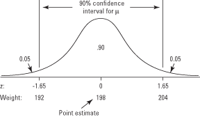
Suppose that you want to find out the average weight of all players on the football team at Landers College. You are able to select ten players at random and weigh them. The mean weight of the sample of players is 198, so that number is your point estimate. Assume that the population standard deviation is σ = 11.50. What is a 90 percent confidence interval for the population weight, if you presume the players' weights are normally distributed?This question is the same as asking what weight values correspond to the upper and lower limits of an area of 90 percent in the center of the distribution. You can define that area by looking up in Table 2 (in "Statistics Tables") the z-scores that correspond to probabilities of 0.05 in either end of the distribution. They are −1.65 and 1.65. You can determine the weights that correspond to these z-scores using the following formula:

What would happen to the confidence interval if you wanted to be 95 percent certain of it? You would have to draw the limits (ends) of the intervals closer to the tails, in order to encompass an area of 0.95 between them instead of 0.90. That would make the low value lower and the high value higher, which would make the interval wider. The width of the confidence interval is related to the confidence level, standard error, and n such that the following are true:
- The higher the percentage of confidence desired, the wider the confidence interval.
- The larger the standard error, the wider the confidence interval.
- The larger the n, the smaller the standard error, and so the narrower the confidence interval.
Figure 1. The relationship between point estimate, confidence interval, and z-score.

Estimating a Difference Score
Imagine that instead of estimating a single population mean μ, you wanted to estimate the difference between two population means μ1 and μ2, such as the difference between the mean weights of two football teams. The statistic has a sampling distribution just as the individual means do, and the rules of statistical inference can be used to calculate either a point estimate or a confidence interval for the difference between the two population means.
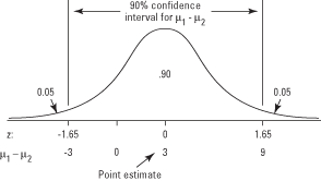
Suppose you wanted to know which was greater, the mean weight of Landers College's football team or the mean weight of Ingram College's team. You already have a point estimate of 198 pounds for Landers's team. Suppose that you draw a random sample of players from Ingram's team, and the sample mean is 195. The point estimate for the difference between the mean weights of Landers's team (μ1) and Ingram's team (μ2) is 198 – 195 = 3.
But how accurate is that estimate? You can use the sampling distribution of the difference score to construct a confidence interval for μ1 – μ2. Suppose that when you do so, you find that the confidence interval limits are (–3, 9), which means that you are 90 percent certain that the mean for the Landers team is between 3 pounds lighter and 9 pounds heavier than the mean for the Ingram team (see Figure 1).
Figure 1. The relationship between point estimate, confidence interval, and z-score, for a test of the difference of two means.

H0: μ1 = μ2
or H0: μ1 – μ2= 0
To reject the null hypothesis of equal means, the test statistic—in this example, z-score—for a difference in mean weights of 0 would have to fall in the rejection region at either end of the distribution. But you have already seen that it does not—only difference scores less than –3 or greater than 9 fall in the rejection region. For this reason, you would be unable to reject the null hypothesis that the two population means are equal. This characteristic is a simple but important one of confidence intervals for difference scores. If the interval contains 0, you would be unable to reject the null hypothesis that the means are equal at the same significance level.
Univariate Tests: An Overview
To summarize, hypothesis testing of problems with one variable requires carrying out the following steps:- State the null hypothesis and the alternative hypothesis.
- Decide on a significance level for the test.
- Compute the value of a test statistic.
- Compare the test statistic to a critical value from the appropriate probability distribution corresponding to your chosen level of significance and observe whether the test statistic falls within the region of acceptance or the region of rejection. Equivalently, compute the p-value that corresponds to the test statistic and compare it to the selected significance level.

The general formula for computing a test statistic for making an inference about a difference between two populations is

The general formula for computing a confidence interval is
observed sample statistic ± critical value × standard error
where observed sample statistic is the point estimate (usually the sample mean), critical value is from the table of the appropriate probability distribution (upper or positive value if z) corresponding to half the desired alpha level, and standard error is the standard error of the sampling distribution. Why must the alpha level be halved before looking up the critical value when computing a confidence interval? Because the rejection region is split between both tails of the distribution, as in a two-tailed test. For a confidence interval at α = 0.05, you would look up the critical value corresponding to an upper-tailed probability of 0.025.


