INVENTORIES - BASICS
Posted by Muhammad Atif Saeed | | Posted in Accounting
Inventory-processing systems relate to the timing of the assessment of inventory. They can be valued on a continuous basis (physical count of inventory will be done after each sale) or periodically (physical count of inventory will be done at the end of each period). For most businesses, continuous revaluation of their inventory is too expensive and generates little value. As a result, most companies evaluate their inventory periodically.
The inventory-costing methods used relate to the way management has decided to evaluate the cost of their inventory, for example, specific identification, average cost, first in first out (FIFO), or last in first out (LIFO). The costing method will have an impact on the estimated value of the inventory on hand and the estimated cost of goods sold (COGS) reported on the income statement.
The valuation method is the process by which the inventory is valued. GAAP requires inventory to be valued at the lower of cost to market (LCM) valuation. Market valuation is defined as replacement cost. The choices made by management with the inventory- processing systems, the inventory-costing method and the valuation method used will affect what is reported on a company's balance sheet, net income statement (profits) and cash flow statement. All these choices should be driven by the application of the matching principle. Unfortunately, these choices are sometimes driven by the owner/management tax implications (usually among private companies), or by the intention to artificially increase a company's profitability (usually among public companies).
Inventory Cost
Inventory cost is the net invoice price (less discounts) plus any freight and transit insurance plus taxes and tariffs. Inventory includes not only inventory on hand but also inventory in transit. Furthermore, inventory does not have to be a finished product to the included.
The cost of inventory can be calculated based on:
1) the specific identification method,
2) the average-cost method,
3) first in, first out (FIFO), and
4) last in, first out (LIFO)
GAAP allows management to use four methods to evaluate inventory. We will use the following example to illustrate each of these methods.
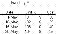
Example: Company ABC purchased these items in May, and sold item 102 and 103 for a total of $300:
 |
1) The Specific-identification Inventory Method
Under this inventory method each unit purchased for resale is identified and accounted for by its invoice. Companies that use this method carry a small number of units.
Cost of goods sold: $75 (ID: 102 and 103)
Ending inventory: $55 (ID: 101 and 104)
Gross profit: $300-$75 = $225
2) Average-cost Method
Under this inventory method the units in inventory are considered as a whole and their cost is averaged out. Companies that use this method carry a large number of units.
Total cost: $130
Average cost: $33 per unit (total cost / total number of units)
Cost of goods sold: $66 ($33*2 units sold)
Ending inventory: $66 ($33*2 units left)
Gross profit: $300-$66 = $234
3) First-in, First-out (FIFO)
Under this inventory method the units that were first purchased are assumed to be sold first.
Cost of goods sold: $65 (ID: 101 and 102)
Ending inventory: $65 (ID: 103 and 104)
Gross profit: $300-$65= $235
4) Last-in, First-out (LIFO)
Under this inventory method the units that were last purchased are assumed to be sold first.
Cost of goods sold: $65 (ID: 103 and 104)
Ending inventory: $65 (ID: 101 and 102)
Gross profit: $300-$65 = $235
Internal Liquidity Ratios
Posted by Muhammad Atif Saeed | | Posted in Accounting
| Current ratio = current assets / current liabilities |
2. Quick RatioThe quick (or acid-test) ratio is a more stringent measure of liquidity. Only liquid assets are taken into account. Inventory and other assets are excluded, as they may be difficult to dispose of.
Formula 7.4
| Quick ratio = (cash+ marketable securities + accounts receivables) current liabilities |
3. Cash Ratio
The cash ratio reveals how must cash and marketable securities the company has on hand to pay off its current obligations.
Formula 7.5
| Cash ratio = (cash + marketable securities)/current liabilities |
4. Cash Flow from Operations Ratio
Poor receivables or inventory-turnover limits can dilute the information provided by the current and quick ratios. This ratio provides a better indicator of a company's ability to pay its short-term liabilities with the cash it produces from current operations.
Formula 7.6
Cash flow from operations ratio = cash flow from operations current liability |
5. Receivable Turnover Ratio
This ratio provides an indicator of the effectiveness of a company's credit policy. The high receivable turnover will indicate that the company collects its dues from its customers quickly. If this ratio is too high compared to the industry, this may indicate that the company does not offer its clients a long enough credit facility, and as a result may be losing sales. A decreasing receivable-turnover ratio may indicate that the company is having difficulties collecting cash from customers, and may be a sign that sales are perhaps overstated.
Formula 7.7
Receivable turnover = net annual sales / average receivables Where:Average receivables = (previously reported account receivable + current account receivables)/2 |
6. Average Number of Days Receivables Outstanding (Average Collection Period)
This ratio provides the same information as receivable turnover except that it indicates it as number of days.
Formula 7.8
Average number of days receivables outstanding = 365 days_ receivables turnover |
7. Inventory Turnover Ratio
This ratio provides an indication of how efficiently the company's inventory is utilized by management. A high inventory ratio is an indicator that the company sells its inventory rapidly and that the inventory does not languish, which may mean there is less risk that the inventory reported has decreased in value. Too high a ratio could indicate a level of inventory that is too low, perhaps resulting in frequent shortages of stock and the potential of losing customers. It could also indicate inadequate production levels for meeting customer demand.
Formula 7.9
Inventory turnover = cost of goods sold / average inventory Where: Average inventory = (previously reported inventory + current inventory)/2 |
8. Average Number of Days in StockThis ratio provides the same information as inventory turnover except that it indicates it as number of days.
Formula 7.10
| Average number of days in stock = 365 / inventory turnover |
9. Payable Turnover RatioThis ratio will indicate how much credit the company uses from its suppliers. Note that this ratio is very useful in credit checks of firms applying for credit. Payable turnover that is too small may negatively affect a company's credit rating.
Formula 7.11
| Payable turnover = Annual purchases / average payables Where: Annual purchases = cost of goods sold + ending inventory - beginning inventory Average payables = (previously reported accounts payable + current accounts payable) / 2 |
10. Average Number of Days Payables Outstanding (Average Age of Payables)
This ratio provides the same information as payable turnover except that it indicates it by number of days.
Formula 7.12
| Average number of days payables outstanding = 365_____ payable turnover |
II. Other Internal-Liquidity Ratios
11.Cash Conversion Cycle
This ratio will indicate how much time it takes for the company to convert collection or their investment into cash. A high conversion cycle indicates that the company has a large amount of money invested in sales in process.
Formula 7.13
| Cash conversion cycle = average collection period + average number of days in stock - average age of payables |
Cash conversion cycle = average collection period + average number of days in stock - average age of payables
12.Defensive Interval
This measure is essentially a worst-case scenario that estimates how many days the company has to maintain its current operations without any additional sales.
Formula 7.14
Defensive interval = 365 * (cash + marketable securities + accounts receivable) projected expenditures Where:Projected expenditures = projected outflow needed to operate the company |
Currency Appreciation and Depreciation
Posted by Muhammad Atif Saeed | | Posted in Economics, Global Economics, Recent
Trade balances are also affected by capital flows. If a nation's economy offers investment opportunities that are relatively better than other nations, then capital will flow into the country. With flexible exchange rates, this capital inflow will tend to increase the value of the nation's currency.
Economic statistics support the hypothesis that trade deficits are associated with investment opportunities and economic growth. Between 1973 and 1982, which was a time of stagnant economic growth for the U.S., trade deficits and net foreign investment were fairly small. As the U.S. economy grew rapidly after the 1982 recession, net foreign investment greatly increased. During the recession of the early 1990s, capital inflow greatly decreased and the current account was actually slightly positive during one of those years. The time between 1993 and 2000 was one of substantial economic growth; net capital inflows greatly increased, which caused the U.S. dollar to appreciate and the current account ran large deficits.
Budget deficits and trade deficits tend to be linkedAn increase in the U.S. government budget deficit will cause an increase in the real interest rate, which causes additional foreign capital to flow into the country. The inflow of foreign currencies will cause the value of the U.S. dollar to increase in relation to other currencies. The increase in value of the U.S. dollar will make U.S. exports relatively less attractive to foreigners and imports into the U.S. will be relatively less expensive; therefore, net exports will go down. The increase in the budget deficit leads to an increase in the trade deficit.
Causes of a Nation's Currency Appreciation or DepreciationFactors that can cause a nation's currency to appreciate or depreciate include:
·Relative Product Prices - If a country's goods are relatively cheap, foreigners will want to buy those goods. In order to buy those goods, they will need to buy the nation's currency. Countries with the lowest price levels will tend to have the strongest currencies (those currencies will be appreciating).
·Monetary Policy - Countries with expansionary (easy) monetary policies will be increasing the supply of their currencies, which will cause the currency to depreciate. Those countries with restrictive (hard) monetary policies will be decreasing the supply of their currency and the currency should appreciate. Note that exchange rates involve the currencies of two countries. If a nation's central bank is pursuing an expansionary monetary policy while its trading partners are pursuing monetary policies that are even more expansionary, the currency of that nation is expected to appreciate relative to the currencies of its trading partners.
·Inflation Rate Differences - Inflation (deflation) is associated with currency depreciation (appreciation). Suppose the price level increases by 40% in the U.S., while the price levels of its trading partners remain relatively stable. U.S. goods will seem very expensive to foreigners, while U.S. citizens will increase their purchase of relatively cheap foreign goods. The U.S. dollar will depreciate as a result. If the U.S. inflation rate is lower than that of its trading partners, the U.S. dollar is expected to appreciate. Note that exchange rate adjustments permit nations with relatively high inflation rates to maintain trade relations with countries that have low inflation rates.
·Income Changes - Suppose that the income of a major trading partner with the U.S., such as Great Britain, greatly increases. Greater domestic income is associated with an increased consumption of imported goods. As British consumers purchase more U.S. goods, the quantity of U.S. dollars demanded will exceed the quantity supplied and the U.S. dollar will appreciate.
Forward Market Calculations
Posted by Muhammad Atif Saeed | | Posted in Economics, Global Economics
The reasons that spreads vary with forward foreign currency quotations are similar to the reasons for the variability of spreads with spot foreign currency quotations. The unique factor associated with spreads for forward foreign currency quotations is that spreads will widen as the length of time until settlement increases. Currency exchange rates would be expected to have a higher range of fluctuations over longer periods of time, which increases dealer risk. Also, as time increases, fewer dealers are willing to provide quotes, which will also tend to increase the spread.
Calculating a Forward Discount or Premium, Expressed as an Annualized Rate.Forward currency exchange rates often differ from the spot exchange rate. If the forward exchange rate for a currency is higher than the spot rate, there is a premium on that currency. A discount exists when the forward exchange rate is lower than the spot rate. A negative premium is equivalent to a discount.
Example: Forward Discount PremiumIf the ninety day ¥ / $ forward exchange rate is 109.50 and the spot rate is ¥ / $ = 109.38, then the dollar is considered to be "strong" relative to the yen, as the dollar's forward value exceeds the spot value. The dollar has a premium of 0.12 yen per dollar. The yen would trade at a discount because its forward value in terms of dollars is less than its spot rate.
The annualized rate can be calculated by using the following formula:
Formula 5.3
Annualized = Forward Price - Spot Price x 12 x 100%Forward Premium Spot Price # of months
forward
Answer:
So in the case listed above, the premium would be calculated as:
Annualized forward premium=
((109.50 - 109.38 ÷ 109.38) × (12 ÷ 3) × 100% = 0.44%
Similarly, to calculate the discount for the Japanese yen, we first want to calculate the forward and spot rates for the Japanese yen in terms of dollars per yen. Those numbers would be (1/109.50 = 0.0091324) and (1/109.38 = 0.0091424), respectively.
So the annualized forward discount for the Japanese yen, in terms of U.S. dollars, would be:
((0.0091324 - 0.0091424) ÷ 0.0091424) × (12 ÷ 3) × 100% = -0.44%
Spot Market Calculations
Posted by Muhammad Atif Saeed | | Posted in Economics, Global Economics
In general, in calculating cross-rates, bid and ask prices will need to be dealt with.
This makes the calculation only slightly more difficult. The following equations should be kept in mind:
Formula 5.2
(FCa / FCb)ask = (FCa / DC)ask ×(DC/FCb)ask
(FCa / FCb)bid = (FCa / DC)bid ×(DC/FCb)bid
Where FCa and FCb are the two foreign currencies and DC is the domestic currency.
Similar equations are used when calculating FCb to FCa exchange rates.
Example: Currency Cross Rates and Ask QuotationsVerifications can be made by checking that (FCb/FCa)ask is equal to the reciprocal of (FCa/FCb)bid, and by checking that (FCb/FCa)bid is equal to the reciprocal of (FCa/FCb)ask.
Suppose you are given the following bid/ask quotations for two foreign currencies against the domestic currency, the U.S. dollar:
Bid Asked¬ / $ 0.9002 0.9023¥ / $ 109.38 109.40
We want to calculate what the ¥ / ¬ bid and ask quotations will be.
Answer:The ¥ / ¬ bid price will be the number of yen the dealer is willing to pay in order to buy one euro. This transaction would be the equivalent of selling yen to purchase dollars (at the bid rate of 109.38), and simultaneously reselling the dollars to purchase euros (at the ask rate of 0.9023). The bid ¥ / ¬ would be calculated as 109.38/0.9023 = 121.22.
The ¥ / ¬ ask price would be the number of yen the dealer wants to receive in exchange for selling one euro. This transaction would be the equivalent of buying yen with dollars (at the 109.40 ask rate) and at the same time buying those dollars with euros, at the 0.9002 bid rate. The transaction could be expressed mathematically as:
Ask ¥ / ¬ = 109.40 / 0.9002 = 121.53
So the resulting dealer quotation would be:
¥ / ¬ = 121.22 - 121.53
| Exam Tip! You can count on getting questions like these on the exam, so make sure that you are comfortable with these types of questions. |
- The Spot Currency Exchange Market - This market involves trades of currencies for immediate delivery. Settlement usually occurs two days after the trade date. Participants in this market want to convert to the other currency relatively quickly. Transactions in the spot market are often used for investments, or to settle commercial purchases of goods.
- The Forward Currency Exchange Market - This market involves contracts for currency exchange in which settlement will take place more than two days after the trade date. While settlement dates are negotiable, standard foreign currency forward contracts usually settle 30, 90 or 180 days after the trade date. If a dealer quotes the 90-day ¥ / $ exchange rate at 109.80-109.83, that means the dealer is willing to commit today to buying dollars for 109.80 yen in 90 days, or to selling dollars at 109.83 yen per dollar 90 days from today.
Trade Efficiency Rule
Posted by Muhammad Atif Saeed | | Posted in Economics, Global Economics
An easy way to determine which country has the comparative advantage is to compare the slopes of the production possibility curves. Suppose you have production possibility curves for two countries with product Y and X, and product Y is placed on the y-axis. The country with the most negative slope for product Y will have the comparative advantage with product Y.
Suppose each country specialized in producing the good for which it had a comparative advantage. The U.S. would produce 50 units of wheat per worker and Great Britain would produce 40 units of steel per worker. The combined world output would be 50 units of wheat and 40 units of steel. With no trade, the combined wheat output is 45 units and the combined steel output is 35 units. Clearly the two countries can benefit from trading with one another - the quantity of wheat produced goes up by five units and the quantity of steel produced goes up by five units. Trading offers more efficient production possibilities.
Production Possibility Curves
Posted by Muhammad Atif Saeed | | Posted in Economics, Global Economics
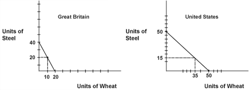 |
The domestic exchange rate within the U.S. for the two goods is 1:1; for each unit of steel produced, the U.S. must give up producing one unit of wheat. We could say that the cost of one unit of steel within the U.S., assuming no international trade, would be one unit of wheat. Similarly, the cost of one unit of wheat would be the loss of one unit of steel.
Great Britain would have a different domestic exchange rate. Its production possibility curve implies that the cost of one unit of steel would be one-half of a unit of wheat. The cost of one unit of wheat would be two units of steel. These costs can be obtained by looking at the slope of the production possibility curve.
If the U.S. and Great Britain both operated as autarkies (self-sufficient nations that do not trade), then each country would operate somewhere on their production possibilities curve. The exact point of production would depend on each country's supply and demand for the goods. For example, these points could be 35 units of wheat and 15 units of steel for the U.S., and 10 units of wheat and 20 units of steel for Great Britain, as illustrated in Figure 5.1.
Peachtree Complete Instructions
Posted by Muhammad Atif Saeed | Thursday, 29 December 2011 | Posted in Accounting, Computer
Cash Flow Computations - Direct Method
Posted by Muhammad Atif Saeed | | Posted in Accounting, feature
The direct method is the preferred method under FASB 95 and presents cash flows from activities through a summary of cash outflows and inflows. However, this is not the method preferred by most firms as it requires more information to prepare.
Cash Flow from OperationsUnder the direct method, (net) cash flows from operating activities are determined by taking cash receipts from sales, adding interest and dividends, and deducting cash payments for purchases, operating expenses, interest and income taxes. We'll examine each of these components below:
- Cash collections are the principle components of CFO. These are the actual cash received during the accounting period from customers.
They are defined as:
Formula 6.7
Cash Collections Receipts from Sales= Sales + Decrease (or - increase) in Accounts Receivable
- Cash payment for purchases make up the most important cash outflow component in CFO. It is the actual cash dispersed for purchases from suppliers during the accounting period.
It is defined as:
Formula 6.8
Cash payments for purchases = cost of goods sold + increase (or - decrease) in inventory + decrease (or - increase) in accounts payable - Cash payment for operating expenses is the cash outflow related to selling general and administrative (SG&A), research and development (R&A) and other liabilities such as wage payable and accounts payable.
It is defined as:
Formula 6.9
| Cash payments for operating expenses = operating expenses + increase (or - decrease) in prepaid expenses + decrease (or - increase) in accrued liabilities |
- Cash interest is the interest paid to debt holders in cash.
It is defined as:
Formula 6.10
| Cash interest = interest expense - increase (or + decrease) interest payable + amortization of bond premium (or - discount) |
- Cash payment for incometaxes is the actual cash paid in the form of taxes. It is defined as:
Formula 6.11
| Cash payments for income taxes = income taxes + decrease (or - increase) in income taxes payable |
Note: Cash flow from investing and financing are computed the same way it was calculated under the indirect method. |
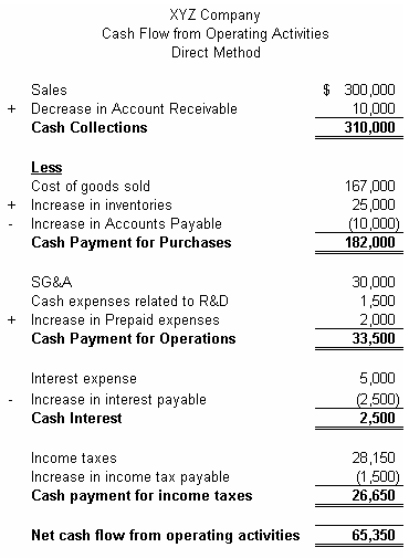
The diagram below demonstrates how net cash flow from operations is derived using the direct method.
 |
Candidates must know the following: |
Cash Flow Computations - Indirect Method
Posted by Muhammad Atif Saeed | | Posted in Accounting, Recent
- The indirect method
- The direct method
The Indirect MethodThe indirect method is preferred by most firms because is shows a reconciliation from reported net income to cash provided by operations.
Calculating Cash flow from OperationsHere are the steps for calculating the cash flow from operations using the indirect method:
- Start with net income.
- Add back non-cash expenses.
- (Such as depreciation and amortization)
- Adjust for gains and losses on sales on assets.
- Add back losses
- Subtract out gains
- Account for changes in all non-cash current assets.
- Account for changes in all current assets and liabilities except notes payable and dividends payable.
In general, candidates should utilize the following rules:
- Increase in assets = use of cash (-)
- Decrease in assets = source of cash (+)
- Increase in liability or capital = source of cash (+)
- Decrease in liability or capital = use of cash (-)
The following example illustrates a typical net cash flow from operating activities:
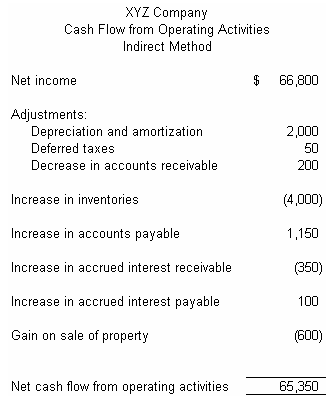 |
Cash Flow from Investment ActivitiesCash Flow from investing activities includes purchasing and selling long-term assets and marketable securities (other than cash equivalents), as well as making and collecting on loans.
Here's the calculation of the cash flows from investing using the indirect method:
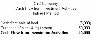 |
Cash Flow from Financing ActivitiesCash Flow from financing activities includes issuing and buying back capital stock, as well as borrowing and repaying loans on a short- or long-term basis (issuing bonds and notes). Dividends paid are also included in this category, but the repayment of accounts payable or accrued liabilities is not.
Here's the calculation of the cash flows from financing using the indirect method:
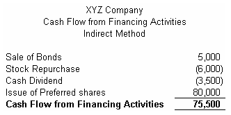 |
Monetary Policy
Posted by Muhammad Atif Saeed | | Posted in Economics, Macro Economics
Price level stability is only a means to a higher goal. That goal is a rising standard of living, which depends upon sustainable growth in real GDP. Whether or not that growth is sustainable depends upon other factors such as technological advances, availability of natural resources, the willingness of people to work, the willingness of people to invest, and political stability. Monetary policy helps to create a stable environment which favors investment and saving.
Achieving Price Level StabilityThe Federal Reserve can quickly affect short-term interest rates, such as three-month T-bills and rates on savings deposits. However, the impact of monetary policy on longer-term interest rates is more moderate and more difficult to predict. Longer-term interest rates are more influenced by the supply and demand for investment funds, as opposed to monetary factors. Secondly, the impact of inflation must be taken into account. For example, suppose an expansionary monetary policy is perceived to be inflationary. The impact of that policy on longer-term interest rates, such as real estate mortgages, will be to raise them.
Expansionary Monetary PolicyAn expansionary monetary policy, if inflationary effects are not anticipated, should lower interest rates, particularly short-term ones. It will also have the effect of reducing velocity, as the opportunity cost of holding money is reduced. Eventually the lower interest rates will induce more personal and business spending to occur so that aggregate demand will increase. This process could take several quarters. Eventually the increased demand will cause nominal and real interest rates to go higher, which will increase the velocity of money. At that point the impact of the expansionary monetary policy will be further amplified.
Expansionary monetary and fiscal policy often assumes that workers will accept lower real wages and that investors will accept lower real rates of return. It is the willingness of workers to accept wages that are lower than what they would normally demand, and the willingness of investors to accept lower real interest rates than normal that causes employment and real production to increase. Nominal wages and interest rates remain the same; inflation is doing the job of cutting real wages and interest rates. Therefore, in order for employment and production to increase, inflation must increase so that real wages and interest rates can go down. This relationship is described by the original Phillips curve, which shows that inflation accompanies lower rates of unemployment.
As long as the public does not understand that inflation has increased, the economy can be moved according to the Phillips curve relationship.
Why would it take time for the public to recognize and adapt to the new rate of inflation? One reason is that some workers may not be able to do anything about it. They may be locked into multi-year labor agreements that do not permit negotiation until the expiration of the labor agreement. Investors and employees might also be subject to money illusion - their attention could be focused on their nominal wages and nominal interest rates, and they may not realize that real wages and interest rates are declining. At some point in time, however, they will recognize that their real buying power (from wages and interest income) has gone down.
Also, they may not immediately see that inflation is occurring. Not all prices go up during times of inflation, so it may hard to see the big picture.
Eventually, the public will understand and adapt to the new inflationary environment and they will seek raises in wages and interest rates in order to bring them back to their old income levels. The economy will move to a long-term equilibrium position in which output and employment return to points where they were before the monetary and fiscal stimulus occurred. The major change will be that prices will be at a higher level.
This makes sense, as we should not expect major benefits to occur just from printing more paper money or running larger government deficits!
Expectations essentially reduce the time that government policymakers can fool the public into accepting cuts in real wage and real interest rates and, therefore, the positive effects of financial and monetary stimulus are moderated.
New Monetarist vs New Keynesian Feedback RulesThere are two famous new feedback rules for monetary policy. Those rules are:
- The Taylor rule is a Keynesian feedback rule that focuses on short-term interest rates. The rule takes into account the target inflation rate, the difference between actual inflation and the target inflation rate, and the difference between real GDP and potential GDP.
- The McCallum rule is a monetarist rule that emphasizes the growth rate of money. It states that the Federal Reserve should target a monetary base growth rate equal to the target inflation rate plus the ten-year moving average of the real GDP growth rate minus the four-year moving average of the monetary base velocity.
The major differences between the rules are:
·Targeting an interest rate versus monetary growth (as usual for Keynesians versus monetarists!).·The Taylor rule provides for a response to fluctuations in real GDP, while the McCallum rule does not.
Discretionary Fiscal Policy and Automatic Stabilizers
Posted by Muhammad Atif Saeed | | Posted in Economics, Macro Economics
Ideally, fiscal policy will be used to increase aggregate demand during recessions and to restrain aggregate demand during boom times. Poorly timed fiscal policy could actually increase inflation and accelerate declines in the economy when the economy has already started to slow down.
One difficulty with proper timing is that forecasting economic activity is not an exact science. There is usually a lag between the time fiscal policy changes are needed and the instance that the need to act is widely recognized. There can also be a substantial amount of time between the time of recognition and the time that fiscal policy changes are actually enacted. Lastly, another difficulty with achieving proper timing is that the impact of a change in fiscal policy may not be felt until six to twelve months after the change has occurred.
Automatic StabilizersAutomatic stabilizers, without specific new legislation, increase (decrease) budget deficits during times of recessions (booms). They enact countercyclical policy without the lags associated with legislative policy changes. Examples include:
·Corporate Profits - Taxes on corporate profits go up substantially during boom times, and decline rapidly during times of recession.
·Progressive Income Taxes - Progressive taxation push people into higher income tax brackets during boom times, substantially increasing their tax bill and reducing government budget deficits (or increasing government surpluses). During recessions, many individuals fall into lower tax brackets or have no income tax liability. This increases the size of the government budget deficit (or reduces the surplus).
· The Unemployment Insurance (UI) Program - This program provides payments to greater numbers of people as unemployment increases during times of recession. At the same time, the taxes that contribute to UI will go down as employment decreases. These two effects will cause the government budget deficit to increase. During boom times, the program will automatically produce surpluses (or reduce deficits) as fewer benefits are paid due to lower unemployment and tax revenues increase due to greater employment.
The Multiplier Effect
Posted by Muhammad Atif Saeed | | Posted in Economics, Macro Economics
| Look Out! In the Keynesian model, government and private investment spending are considered to be autonomous while consumption is not because it is a function of income. |
Why is there a multiplier effect?Suppose a large corporation decides to build a factory in a small town and that spending on the factory for the first year is $5 million. That $5 million will go to electricians, engineers and other various people building the factory. If MPC is equal to 0.8, those people will spend $4 million on various goods and services. The various business and individual receiving that $4 million will in turn spend $3.2 million and so on.
If the marginal propensity to consume is equal to 0.8 (4 / 5), then the multiplier can be calculated as:
Multiplier = 1 / (1 - MPC) = 1 / (1 - 0.8) = 1 / 0.2 = 5
As a result of the multiplier effect, small changes in investment or government spending can create much larger changes in total output. A positive aspect of the multiplier effect is that macroeconomic policy can effect substantial improvements with relatively small amounts of autonomous expenditures. A negative aspect is that a small decline in business investment can trigger a larger decline in business activity and, thereby, create instability.
The previously mentioned formula for calculating the multiplier is a simplified one. Leakages (money spent, but not on domestic goods or domestic services) reduce the size of the multiplier. Examples of leakages include taxes and imports.
Another important point is that the multiplier effect takes time to work; months must pass before even half of the total multiplier effect is felt. Also, keep in mind that the multiplier effect can cause idle resources to be moved into production. If unemployment is widespread, then there should be little impact on resource prices.
Posted by Muhammad Atif Saeed | | Posted in Economics, Macro Economics
Potential GDPThe GDP that results from an economy operating at full employment with full utilization of capital is called potential GDP.
A reduction in after-tax wages will occur with the enactment of an income tax. The supply curve of labor will therefore shift up and to the left. The new equilibrium quantity of labor hired will be less than what would have occurred with potential GDP. There will be a "wedge" between before-tax and after-tax wage rates. Taxes on expenditure increase the size of the "wedge" and further reduce employment.
Keynesians argue that if output is less than what would occur at full employment, fiscal policy should be used to stimulate aggregate demand.
There are three major ways in which fiscal policy affects aggregate demand:
1.Business Tax Policy - Business taxes can change the profitability of businesses and the amount of business investment. Lowering business taxes will increase aggregate demand and business investment spending.
2.Government Spending - Government can directly increase aggregate demand by increasing its spending.
3.Tax Policy for Individuals - Lowering taxes will increase disposable personal income and increase consumption spending.
From the Keynesian viewpoint, fiscal policy should be used to increase aggregate demand when an economy is operating at below full-employment levels. Ideally, the economy will be guided to output at the level of full employment.
If aggregate demand exceeds aggregate supply and output is at full-employment levels, fiscal policy should be used to reduce aggregate demand. This will push the economy to a point of noninflationary equilibrium.
The Supply Side Model is an economic theory holding that bolstering an economy's ability to supply more goods is the most effective way to stimulate economic growth. Supply-side theorists advocate income tax reduction because it increases private investment in corporations, facilities, and equipment.
The Laffer curve shows the relationship between tax rates and tax revenue.
Figure 4.6: The Laffer Curve
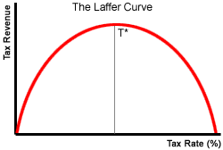 |
Governments would like to be at point T*, because it is the point at which the government collects maximum amount of tax revenue while people continue to work hard. This would theoretically be the point at which potential GDP is maximized.
Supply-side economists believe that high marginal tax rates, such as those experienced in the U.S. in the 1970s, diminished aggregate production without raising substantial amounts of additional tax revenue. Tax cuts during the 1980s (the Reagan presidency) are believed to have induced strong increases in supply, particularly with regards to high-income earners. Supporters of the 2001 U.S. tax cuts, which reduced the top marginal tax rates, believe that the cuts have increased economic growth through better supply-side incentives.
Tax policy also has consequences at a global level. Ireland has significantly reduced its personal and corporate tax rates; during the 1990s its growth rate was much higher than the rest of Europe. There is an association with high European tax rates and slow rates of economic growth.
·Government spending and tax policy will generate either a budget surplus or a deficit, which will in turn mean that the government sector will either contribute towards financing investment or "crowd out" private investment.·Tax policy will affect the amount saved. Taxes on interest earned will decrease the incentive to save and create a wedge between the after-tax interest earned by savers and the interest rate paid by firms.
Generational Effects of Fiscal PolicyCurrent fiscal policy impacts the amount of taxes that future citizens will pay. If the government runs up long-term budget deficits, then future generations will need to pay higher taxes in order to pay the interest. Similarly, future generations will pay lower taxes if the government creates budget surpluses. Economists have created systems which examine the lifetime taxes and benefits associated with generations or age groups. Those systems are referred to as generational accounting.
A government that chronically runs deficits will, at some point in time, have to address that imbalance. This fiscal imbalance will need to be addressed with higher tax revenues and/or reduced government spending.An imbalance is also created when the government benefits received by one generation exceed the taxes paid by that generation. For example, initial recipients of Social Security in the United States received far more benefits than they paid in taxes. Such imbalances are referred to as generational imbalances.Future generations will need to pay more taxes, or receive less benefits, in order to address this imbalance. Fiscal policy therefore transfers benefits according to age; it also determines how much each generation will pay the government.
Inflation
Posted by Muhammad Atif Saeed | | Posted in Economics, Macro Economics
Inflation vs. Price-LevelThe term price-level refers to the prices that must be paid in order to acquire a basket of good and services. The phenomenon of inflation refers to a continual rise of the price-level. When inflation occurs, the purchasing power of a unit of money (the dollar in the United States) is declining.
The inflation rate is calculated by comparing the price level in one time period to the price level of a previous period. Suppose the price level is currently 110, and the price level of the previous year is 100. The annual rate of inflation would then be 10%.
The inflation rate in general can be stated as:
Formula 4.6
Inflation Rate = ((P1 - P0) / P0) X 100
P1 is the price level of the later time period, and P0 is the price level of the previous time period.
Causes of Inflation
Two main types of impulses for inflation in an economy include:
·Demand-pull - aggregate demand rising more rapidly than aggregate supply
·Cost-push - there is a decrease in aggregate supply
Factors creating a demand-pull inflation include an:
·Increase in government spending
·Increase in the supply of money
·Increase in the price level in the rest of the world - if prices increase in other countries, residents of those countries will want to buy goods from domestic producers; i.e., exports will increase
The main factors which induce a cost-pull inflation include an:
·Increase in wage rates
·Increase in raw material costs
Demand-pull inflation represents an increase in aggregate demand, which will shift the aggregate demand curve to the right. Cost-push inflation will involve the aggregate supply curve shifting to the left.Both result in higher price levels.
Unanticipated InflationUnanticipated inflation in the labor market will cause workers to work for less wages then what they would knowingly work for. Employers may get higher profits due to the higher prices. The result will be a transfer of income from workers to employers. There is also a possibility that employment will be higher than "full employment".
Unanticipated inflation in the financial capital market also begets a transfer of income. In this case, borrowers gain at the expense of lenders. The amount of borrowing and lending will not be optimal, as lenders will unwittingly loan out too much funds.
Anticipated vs. Unanticipated InflationInflation that comes as a surprise to most people is called unanticipated inflation. If changes in price levels are widely anticipated, then that inflation is referred to as anticipated inflation. In general, steady rates of inflation can be anticipated successfully by economic decision makers.
There are many harmful consequences to inflation. Some of the consequences include:
- Individuals Apply their Efforts to Protecting Themselves from Inflation Instead of to Production - People will spend a great deal of time and money acquiring information about how to protect themselves (and/or profit) from inflation. Capital flows towards speculative assets such as gold and art objects, instead of productive investments such as buildings and machinery and the incentive to speculate instead of work increases.
- Inflation Increases the Risk of Investments - Wild fluctuations in price levels make forecasting future earnings more difficult; this tend to discourage investment.
- The Information Delivered by Prices is Distorted by Inflation - Some price changes are restrained by long-term contracts, while others respond quickly to changes in the general price level.
- Unanticipated inflation can change relative prices. These distorted prices may provide poor signals to producers and resource suppliers.
Money, Interest, Real GDP, and the Price Level
Posted by Muhammad Atif Saeed | | Posted in Economics, Macro Economics
- To conduct transactions
- For precautionary reasons, such as to meet emergencies, such as unexpected medical bills
- As a store of value
Holding money has an opportunity cost in the sense that the money could be invested elsewhere and earn interest. Even if the money is held in an interest-earning checking account, a higher rate of interest could be earned by purchasing financial instruments such as bonds.
As the rate of interest goes higher, the opportunity cost of money increases. So as interest rates go up (down), people will be less (more) willing to hold money.
The supply of money is usually determined by the Central Bank (Canada) or the Federal Reserve (U.S.) and the targeted supply of money is not directly related to the interest rate.
A graph for the supply and demand for money, as a function of the interest rate, would appear similar to figure 4.4 on the following page.
Figure 4.4: The Supply and Demand for Money
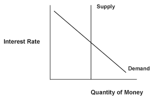 |
Note that this demand curve assumes other relevant factors are held constant. If the quantity of goods produced increases and/or the price level increases, the demand for money will increase. This causes the demand curve to shift to the right. If economic activity declines and/or prices go down, then demand for money will decrease.
Changes in the availability of financial instruments are also changing the demand for money over time. The widespread availability of credit cards has reduced the amount of money that households need to keep on hand.
Determining Interest Rates
Interest rates are determined by the interaction of the quantity supplied and the quantity demanded of money. The quantity supplied of money is determined by the actions of the central bank and the banking system. Suppose that the interest rate is too high in the sense that the quantity of money supplied is greater than the quantity of money demanded. People will respond by purchasing bonds, in which case money will be reduced. The greater demand for bonds will push interest rates down, towards equilibrium.
Short and Long-run Effects of Money on Real GDP
·Short-Run, Anticipated - If individuals correctly anticipate inflation, in the short-run an expansionary (restrictive) monetary policy will increase (decrease) prices. Real output and employment will remain the same. Nominal interest rates will increase while real interest rates will stay the same.
·Long-Run, Anticipated - Expansionary (restrictive) monetary policy will increase (decrease) the rate of inflation and increase (decrease) nominal interest rates. Real interest rates, employment levels and real output are not affected by monetary policy.
·Short-Run, Unanticipated - Unanticipated expansionary monetary policy, assuming the economy is not at full employment, will somewhat increase prices, increase real output and reduce real interest rates. Unanticipated restrictive monetary policy will increase real interest rates, decrease the inflation rate, reduce employment and reduce output. This type of policy is appropriate when the economy is operating at greater than full employment.
·Long-Run, Unanticipated - Expansionary monetary policy will lead to higher inflation and nominal interest rates while real interest rates, real output and real employment will not be positively impacted. An important point to remember is that, in the long run, inflation is the primary effect of expansionary monetary policy.
The Banking System
Posted by Muhammad Atif Saeed | | Posted in Economics, Macro Economics
1.Commercial banks
2.Thrift institutions such as credit unions, savings and loan associations (S&Ls), and savings banks. Credit unions are cooperative organizations, usually restricted to employees of a particular firm or government entity. The savings banks and S&Ls have historically focused their loan activities to the real estate mortgages.
3.Money market mutual funds offer bank-like features. Shareholders of these funds are allowed to write checks against these funds. However, these funds do have restrictions. The mutual funds specify minimum check amounts such as $250.
Their main economic functions include providing liquidity, lowering the cost of borrowing money, and pooling the risk associated with lending money.
All of these institutions make money by charging more for loans than what they pay for deposits, and they are all subject to substantial regulation. Major areas of concern for regulation include reserve requirements, capital requirements, lending rules, and deposit rules. For example, in the past, only commercial banks could offer checking accounts, and savings banks could only offer saving accounts. Those restrictions were relaxed in the 1980s.
Money market mutual funds have been a major force in providing competitive interest rates to short-term depositors. Technological innovation has been a major force in providing new services to customers. For example, crediting interest on a daily basis was not feasible before the advent of modern computer technology.
The Fractional Reserve Banking SystemA fractional reserve banking system exists when the amount of reserves banks must keep on hand is less than the amount of their deposits. In the U.S., banks must keep a fraction of their assets as bank reserves - cash plus deposits with the Federal Reserve, which is the nation's central bank. Banks issue loans with the funds that are not held in reserve; in doing so, they expand the nation's money supply.
The Required Reserve RatioThe required reserve ratio is the percentage of a particular liability category (to the bank), such as savings accounts, that must be held as reserves. If someone deposits $10,000 at a bank and there is a 20% reserve requirement, the bank must keep $2,000 as reserves and can loan out only $8,000. If the reserve requirement is 10%, the bank could loan out $9,000. The $9,000 that is loaned out can be deposited at the original bank or at another bank; 90% of that $9,000, which is $8,100, can then be loaned out. This process continues until the amount of money supply generated is equal to $10,000 × (1 / .1) = $100,000.
The Actual and Potential Deposit Expansion MultipliersThe potential deposit expansion multiplier is the reciprocal of the required reserve ratio. If the required reserve ratio is 5% (.05), the potential deposit expansion multiplier is equal to 1 / .05 = 20.
The actual deposit expansion multiplier is less than the potential deposit expansion multiplier for two reasons:
·Banks may not loan out all available funds (i.e. they may have excess reserves, which are reserves that exceed required reserves)
·Recipients of loans may not deposit the proceeds; they may instead decide to hold them as currency


