Measures of Central Tendency

Measures of central tendency are numbers that tend to cluster around the “middle” of a set of values. Three such middle numbers are the mean, the median, and the mode.
For example, suppose your earnings for the past week were the values shown in Table 1.

Mean

You could express your daily earnings from Table 1 in a number of ways. One way is to use the average, or mean, of the data set. The arithmetic mean is the sum of the measures in the set divided by the number of measures in the set. Totaling all the measures and dividing by the number of measures, you get $1,000 ÷ 5 = $200.

Median

Another measure of central tendency is the median, which is defined as the middle value when the numbers are arranged in increasing or decreasing order. When you order the daily earnings shown in Table 1, you get $50, $100, $150, $350, and $350. The middle value is $150; therefore, $150 is the median.
If there is an even number of items in a set, the median is the average of the two middle values. For example, if we had four values—4, 10, 12, and 26—the median would be the average of the two middle values, 10 and 12; in this case, 11 is the median. The median may sometimes be a better indicator of central tendency than the mean, especially when there are outliers, or extreme values.

Mode

Another indicator of central tendency is the mode, or the value that occurs most often in a set of numbers. In the set of weekly earnings in Table 1, the mode would be $350 because it appears twice and the other values appear only once.

Notation and formulae

The mean of a sample is typically denoted as (read as x bar). The mean of a population is typically denoted as μ (pronounced mew). The sum (or total) of measures is typically denoted with a Σ. The formula for a sample mean is
where n is the number of values.

Mean for grouped data

Occasionally, you may have data that consist not of actual values but rather of grouped measures. For example, you may know that, in a certain working population, 32 percent earn between $25,000 and $29,999; 40 percent earn between $30,000 and $34,999; 27 percent earn between $35,000 and $39,999; and the remaining 1 percent earn between $80,000 and $85,000. This type of information is similar to that presented in a frequency table. Although you do not have precise individual measures, you still can compute measures for grouped data, data presented in a frequency table.
The formula for a sample mean for grouped data is
where x is the midpoint of the interval, f is the frequency for the interval, fx is the product of the midpoint times the frequency, and n is the number of values.
For example, if 8 is the midpoint of a class interval and there are ten measurements in the interval, fx = 10(8) = 80, the sum of the ten measurements in the interval.
Σ fx denotes the sum of all the products in all class intervals. Dividing that sum by the number of measurements yields the sample mean for grouped data.
For example, consider the information shown in Table 3.
Substituting into the formula:
Therefore, the average price of items sold was about $15.19. The value may not be the exact mean for the data, because the actual values are not always known for grouped data.

Median for grouped data

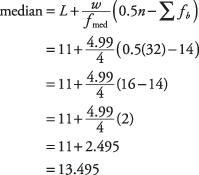
As with the mean, the median for grouped data may not necessarily be computed precisely because the actual values of the measurements may not be known. In that case, you can find the particular interval that contains the median and then approximate the median.
Using Table 3, you can see that there is a total of 32 measures. The median is between the 16th and 17th measure; therefore, the median falls within the $11.00 to $15.99 interval. The formula for the best approximation of the median for grouped data is
where L is the lower class limit of the interval that contains the median, n is the total number of measurements, w is the class width, f_medis the frequency of the class containing the median, and Σ f_b is the sum of the frequencies for all classes before the median class.
Consider the information in Table 4.
As we already know, the median is located in class interval $11.00 to $15.99. So L = 11, n = 32, w = 4.99, f_med = 4, and Σ f_b = 14.
Substituting into the formula:

Symmetric distribution

In a distribution displaying perfect symmetry, the mean, the median, and the mode are all at the same point, as shown in Figure 1.

Skewed curves

As you have seen, an outlier can significantly alter the mean of a series of numbers, whereas the median will remain at the center of the series. In such a case, the resulting curve drawn from the values will appear to be skewed, tailing off rapidly to the left or right. In the case of negatively skewed or positively skewed curves, the median remains in the center of these three measures.
Figure 2 shows a negatively skewed curve.
Figure 3 shows a positively skewed curve.

Measures of Variability

Measures of central tendency locate only the center of a distribution of measures. Other measures often are needed to describe data.

For example, consider the two sets of numbers presented in Table 1.
The mean, the median, and the mode of each employee's daily earnings all equal $200. Yet, there is significant difference between the two sets of numbers. For example, the daily earnings of Employee A are much more consistent than those of Employee B, which show great variation. This example illustrates the need for measures of variation or spread.

Range

The most elementary measure of variation is range. Range is defined as the difference between the largest and smallest values. The range is a single number. To say that the range is from $190 to $200, although informative, is not really a correct use of the term. The range for Employee A is $210 – $190 = $20; the range for Employee B is $400 – $0 = $400.

Deviation and variance

The deviation is defined as the distance of the measurements away from the mean. In Table 1, Employee A's earnings have considerably less deviation than Employee B's do. The variance is defined as the sum of the squared deviations of n measurements from their mean divided by ( n – 1).
So, from Table 1, the mean for Employee A is $200, and the deviations from the mean are as follows:
The squared deviations from the mean, therefore, are the following:
The sum of these squared deviations from the mean equals 252. Dividing by ( n – 1), or 8 – 1, yields . So, the variance is 36.
For Employee B, the mean is also $200, and the deviations from the mean are as follows:
The squared deviations, therefore, are the following:
The sum of these squared deviations equals 217,000. Dividing by ( n – 1) yields .
Although they earned the same totals, there is significant difference in variance between the daily earnings of the two employees.

Standard deviation

The standard deviation is defined as the positive square root of the variance; thus, the standard deviation of Employee A's daily earnings is the positive square root of 36, or 6. The standard deviation of Employee B's daily earnings is the positive square root of 31,000, or about 176.

Notation

s² denotes the variance of a sample.
σ² denotes the variance of a population.
s denotes the standard deviation of a sample.
σ denotes the standard deviation of a population.

Empirical rule: The normal curve

One practical significance of the standard deviation is that, with mound-shaped (bell-shaped) distributions, the following rules apply:

• The interval from one standard deviation below the mean to one standard deviation above the mean contains approximately 68 percent of the measurements.
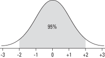
• The interval from two standard deviations below the mean to two standard deviations above the mean contains approximately 95 percent of the measurements.
• The interval from three standard deviations below the mean to three standard deviations above the mean contains approximately all the measurements.

These mound-shaped curves usually are called normal distributions or normal curves (see Figures 1, 2, and 3).

Shortcut formulae

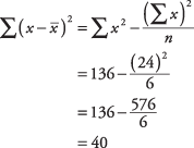
A shortcut method of calculating variance and standard deviation requires two quantities: sum of the values and sum of the squares of the values.
For example, using these six measures: 3, 9, 1, 2, 5, and 4:
The quantities are then substituted into the shortcut formula to find .
The variance and standard deviation are now found as before:

Percentile

The Nth percentile is defined as the value such that N percent of the values lie below it. So, for example, a score of 5 percent from the top score would be the 95th percentile because it is above 95 percent of the other scores (see Figure 4).

Quartiles and interquartile range

The lower quartile ( Q₁) is defined as the 25th percentile; thus, 75 percent of the measures are above the lower quartile. The middle quartile ( Q₂) is defined as the 50th percentile, which is, in fact, the median of all the measures. The upper quartile ( Q₃) is defined as the 75th percentile; thus, only 25 percent of the measures are above the upper quartile.
The interquartile range ( IQR) is the value for Q₃ – Q₁. Like the range, it is a single value.
Figure 5 illustrates the locations of the median and the quartiles for a set of 20 test scores.

Measurement Scales

Different measurement scales allow for different levels of exactness, depending upon the characteristics of the variables being measured. The four types of scales available in statistical analysis are

• Nominal: A scale that measures data by name only. For example, religious affiliation (measured as Christian, Jewish, Muslim, and so forth), political affiliation (measured as Democratic, Republican, Libertarian, and so forth), or style of automobile (measured as sedan, sports car, SUV, and so forth).
• Ordinal: A scale that measures by rank order only. Other than rough order, no precise measurement is possible. For example, medical condition (measured as satisfactory, fair, poor, guarded, serious, and critical); socioeconomic status (measured as lower class, lower-middle class, middle class, upper-middle class, upper class); or military officer rank (measured as lieutenant, captain, major, lieutenant colonel, colonel, general). Such rankings are not absolute but rather relative to each other: Major is higher than captain, but we cannot measure the exact difference in numerical terms. Is the difference between major and captain equal to the difference between colonel and general? We cannot say.
• Interval: A scale that measures by using equal intervals. Here you can compare differences between pairs of values. The Fahrenheit temperature scale, measured in degrees, is an interval scale, as is the centigrade scale. The temperature difference between 50°C and 60°C (10 degrees) equals the temperature difference between 80°C and 90°C (10 degrees). Note that the 0 in each of these scales is arbitrarily placed, which makes the interval scale different from ratio.
• Ratio: Similar to an interval scale, a ratio scale includes a 0 measurement that signifies the point at which the characteristic being measured vanishes (absolute zero). For example, income (measured in dollars, with 0 equal to no income at all), years of formal education, items sold, and so forth, are all ratio scales.

About the Author

By Muhammad Atif Saeed on 06:57. Filed under feature , Statistics . Follow any responses to the RSS 2.0. Leave a response