Published On:Sunday, 27 November 2011
Posted by Muhammad Atif Saeed
Break Even Analysis
Management Accounting
“The process of identifying, measuring and communicating economic information to permit informed judgments and decisions by users of information”
STEPS OF DECISION MAKING PROCESS
- Identify objective
- Search for alternative course of action
- Gather data about alternative
- Select alternative course of action
- Implement the decision
- Compare actual and planned outcomes
- Respond to difference from plan
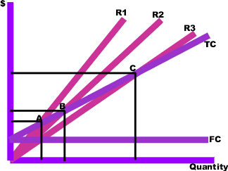
Break even analysis
• break-even analysis provides a simple means of measuring profits and losses at different levels of output
• sales revenues and total costs are analysed for each different level of production
• analysis is normally done graphically using a break-even chart
Margin of Safety: the difference between actual output and the break-even output is known as the margin of safety
Break even point
• the point at which total costs are covered and no profit or loss is made is called the break-even point
• the break-even point is where the total revenue and total cost lines intersect on the chart
BEP= Fixed Cost .
Contribution per unit
Example
Assuming that a product has a selling price of £6. Variable costs are £1 per unit and fixed costs are £50,000 per year
Calculate the number of units that a firm must sell in order to break-even
Answer - £50,000 = 10000 units
£5
Use of Break Event Analysis
- to calculate the minimum amount of sales required in order to be able to break even
- to see how changes in output, selling price or costs will affect profit levels
- to calculate the level of output required to reach a certain level of profit
- to allow various scenarios (what-if) to be tested out
- to aid forecasting and planning
Limitation of Break Even Analysis
- it’s accuracy depends upon the accuracy of the data used
- forecasting the future is difficult, especially long term
- it assumes there is a simple relationship between variable costs and sales
- sales income does not necessarily rise in a constant relationship to sales volume
- external constraints have to be recognised
- Production and sales are assumed to be the same and therefore the consequences of any increase in stock levels or de stocking is ignored.
The total revenue line is curvilinear because to increase the number of units sold the selling price has to be reduced. The line therefore increases at a decreasing rate and eventually begins to decline as the benefits of increased sale volume are outweighed by the adverse effect of price reduction
The total line cost shows economies of a scale at first( unit cost decreases as output increases) but then returns upwards as diminishing returns set in.
|
Factors effecting cost behavior
1. Volume or activity level- Selling cost may vary with the volume, size weight or value of sale, whilst production costs may vary with the number of units produced or the number of hours worked.
2. Nature of the cost- The nature of cost will often aid in predicting its likely amount. If maintenance of machines is single overhaul each year, then maintenance cost is fixed cost.
3. The existence of spare capacity
4. Other factors- Degree of efficiency
| Behavior of Cost (within the relevant range) | ||
| Cost | In Total | Per Unit |
| Variable | Total variable cost changes as activity level changes. | Variable cost per unit remains the same over wide ranges of activity. |
| Fixed | Total fixed cost remains the same even when the activity level changes. | Fixed cost per unit goes down as activity level goes up. |
Assumption of CVP Analysis
- Selling price is constant.
- Cost are linear can accurately divided into variable fixed elements. The variable element is constant per unit, and the fixed element is constant in total over the entire relevant range.
- in multi product companies the sale mix is constant.
- in manufacturing companies, inventories do not change. The number of units produced equals the number of units sold.
FORMULAS SECTION 1
1) Sales = Total cost + Profit = Variable cost + Fixed cost + Profit
2) Total Cost = Variable cost + Fixed cost
3) Variable cost = It changes directly in proportion with volume
4) Variable cost Ratio = {Variable cost / Sales} * 100
5) Sales – Variable cost = Fixed cost + Profit
6) Contribution = Sales * P/V Ratio
7) Profit Volume Ratio [P/V Ratio]:-
- {Contribution / Sales} * 100
- {Contribution per unit / Sales per unit} * 100
- {Change in profit / Change in sales} * 100
- {Change in contribution / Change in sales} * 100
8) Break Even Point [BEP]:-
- Fixed cost / Contribution per unit [in units]
- Fixed cost / P/V Ratio [in value] (or) Fixed Cost * Sales value per unit
(Sales – Variable cost per unit)
9) Margin of safety [MOP]
- Actual sales – Break even sales
- Net profit / P/V Ratio
- Profit / Contribution per unit [In units]
10) Sales unit at Desired profit = {Fixed cost + Desired profit} / Cont. per unit
11) Sales value for Desired Profit = {Fixed cost + Desired profit} / P/V Ratio
12) At BEP Contribution = Fixed cost
13) Variable cost Ratio = Change in total cost * 100
Change in total sales
Indifference Point = Point at which two Product sales result in same amount of
profit
= Change in fixed cost (in units)
Change in variable cost per unit
= Change in fixed cost (in units)
Change in contribution per unit
= Change in Fixed cost (in Rs.)
Change in P/Ratio
= Change in Fixed cost (in Rs.)
Change in Variable cost ratio
15) Shut down point = Point at which each of division or product can be closed
= Maximum (or) Specific (or) Available fixed cost
P/V Ratio (or) Contribution per unit
If sales are less than shut down point then that product is to shut down.
16) Degree of operating leverage = contribution margin .
Net operating income
Equation of regression line of Y on X is of the form
Regression is used to predict a linear relationship between two variables. Unlike the high low method it uses all past data to calculate the line of best fit. It derives a line of best fit by a statistical method.
Interpolation and extrapolation
Calculation of value within the known range is called interpolation and outside range can be calculated is called extrapolation. In extrapolation it is assumed all other costs remain the same.
Y = a + bx
a= ∑y - b∑x
n n
b= n∑xy - ∑x∑y
n∑x2 - (∑x)2
Correlation
Through regression analysis it is possible to derive a linear relationship between two variables, such as total cost and activity level and estimate a formula for the line. However, this does not measure the degree of correlation between two variables. Correlation measures how strong the connection is between the two variables. When correlation is strong, the estimated line of best fit should be more reliable. On the other hand if correlation is weak, the line of best fit calculated by linear regressin might be insufficiently reliable.
If r = + 1 means a perfect positive correlation
If r = 0 means no correlation
If r = - 1 means a perfect negative correlation
It must be realized that r only measures the amount of linear correlation i.e. tendency to a straight line relationship. It is quite possible to have strong non-linear correlation and yet have a value of r close to zero.
r= n∑xy - ∑x∑y .
Coefficient of determination
Is the square of the coefficient of correlation, and so is denoted by r2.
The coefficient of determination is a measure of how much of the variation in the dependent variable is “explained” by the variation of independent variable. When x is output volume and y is total cost, the coefficient of determination will show how much of the variations in total cost can be explained by variations in activity level
Spurious correlation
There is big danger involved in correlation analysis. Two variable, when compared may show a high degree of correlation but they may still have no direct connection. Such correlation is termed as spurious or nonsense correlation. E.g. number of television licenses and the number of admission to mental hospital.
Cost Centre
CIMA “A production or service location, function, activity or item of equipment for which cost accumulated” A cost centre is used as a “collecting place” for costs.